Overview and Table of Contents

Large Langage Models (or LLMs) are all the rage these days. From AI assistants that can write our emails and do our homework for us to reinvigorated conversations about AGI and what it means to be conscious, LLMs have truly transitioned to center stage in the year 2023. Heck, LLMs can even write blog post introductions: “In this post, we’ll look at an example of how LLMs can be leveraged to extract knowledge, glean insights and engage interactive dialogues with repositories of information, such as academic papers and legal documents.”. Get ready to chat with your documents!

1. Introduction to LLM Pipelines
2. Chaining Frameworks: Haystack & LangChain
   1. Haystack
   2. LangChain
   3. Compare & Contrast
3. Pipeline Components: Putting the Pieces Together
   1. Loading Documents
   2. Document Splitters
   3. Words to Vectors: Embeddings & Vectorstores
      1. Bag of Words
      2. Term Frequency - Inverse Document Frequency
      3. Word Embeddings
   4. Retrievers
      1. Similarity Search
      2. Locality Sensitive Hashing
   5. Rankers: Bi-Encoders vs Cross-Encoders
   6. Readers
   7. Generative Pipelines
4. LLM Pipeline Use-Cases
5. CLI Application
6. References

Introduction to LLM Pipelines

Computers represent information as yesses and nos, 1s and 0s, but most human beings don’t speak binary to each other every day. How, then, do people communicate with computers? From low-level languages like assembly to high-level abstractions like Python, computer science has produced a number of different paradigms that enable just that. We call them programming languages. But the extent to which programming languages enable “communication” is restricted. Namely, communications to the machine are required to follow strict rules (syntax) in order to be understood properly (interpreted or compiled) and any communication from the machine must first have been explicitly instructed by the programmer. So, how on earth do applications like ChatGPT exist?!

Enter natural language processing (NLP) and LLM pipelines. The goal of NLP is to endow a machine with the ability to understand and utilize natural language, that is: the means by which we communicate with other people (plain old English, for example). This is a tall ask, but modern frameworks like LangChain and Haystack put it within reach for those with some Python experience and minimal exposure to concepts in modern NLP. In the following sections, we’ll explore some foundational NLP & LLM concepts, along with Haystack and LangChain building blocks, all directed towards the aim of developing applications that enable us to chat with our documents. Everything we do is based on open source technologies and can be run entirely locally. That means, no sending your data to APIs and no paywalls!

Chaining Frameworks: Haystack & LangChain

It’s never been easier and never been less intimidating to build powerful NLP applications. Haystack and LangChain are part of a new wave of tools for interfacing with LLMs and related infrastructure that have made great advancements in abstraction. The rest of this post will be a mixture of high-level concepts, a little bit of theory and examples of how to implement those theories and concepts using these frameworks. So, let’s familiarize ourselves a bit.

Haystack

Haystack describes itself as an “open source Python framework by deepset for building custom apps with large language models “. It utilizes three main types of objects:

1. Components or Nodes: “fundamental building blocks that can perform tasks like document retrieval, text generation, or summarization.”
2. Pipelines: “structures made up of components, such as a Retriever and Reader, connected to infrastructure building blocks, such as a DocumentStore (for example, Elasticsearch or Weaviate) to form complex systems.”
3. Agents: makes use of tools (like pipeline components or whole pipelines) to resolve complex tasks.

For our purposes, we’ll need only the first two. We’ll talk more about each object we use as we come to it, but you can find, still, more info in Haystack’s documentation.

LangChain

Similar to Haystack, LangChain describes itself as “a framework for developing applications powered by language models.” And the similarities don’t end there. They share very similar interfaces, as well. The analogous objects here are:

1. Components: “abstractions for working with language models, along with a collection of implementations for each abstraction.”
2. Chains: “a structured assembly of components for accomplishing specific higher-level tasks.”
3. Agents: lets “chains choose which tools to use given high-level directives.”

Again, we’ll only be utilizing the first two, with more implementation details to come. Checkout LangChain’s documentation for more information.

Compare & Contrast

Two frameworks with similar functionality and similar interfaces … naturally, the questions arise:

• “Is one ‘better’ than the other?”
• “Which should we use?” and
• “Why are we using both?”.

If you like straight answers, apologies in advance because my honest takes are:

• “It depends.”
• “It depends.” and
• “… because it depends.”.

I’ll explain more as we start digging into the meat of the project. Let’s dive in.

Pipeline Components: Putting the Pieces Together

By the end of this post, we’ll have looked at how to implement three different types of pipelines (or chains): ‘generative’, ‘retriever-reader’ and ‘retriever-ranker’. But before we start discussing any of these, we need to talk ‘preprocessing’. Namely, we need to figure out how to take documents sitting in a directory and prepare them for consumption by a pipeline. Well, they say a picture is worth a thousand words, right? Here’s an example of what a preprocessing workflow might look like. This is the workflow utilized in Docs2Chat.

graph LR;
    A[/Some Document/]
    B[/Another Document/]
    C[/One More Document/]
    D[Document Loader]
    E[Document Splitter]
    F[(Vectorstore: Embeddings)]

    A & B & C --> D
    D --> E --> F

Don’t wory, if you’re not already familiar with the components in the diagram; we’ll elaborate on each of them in the following sections. To get started, let’s ‘load’ some documents.

Loading Documents

Documents are represented in both Haystack and LangChain by Document objects. Each framework has a slightly different implementation, but they are very similar and we’ll see later how easy it is to go back and forth between them.

In Haystack, the relevant loading objects are called FileConverters. You’ll find ten implementations covering a number of potential file types, including Markdown, PDFs, DOCX files, etc.. It’s a nice collection and not terribly difficult to combine them into a single ‘load any, depending on the type’ process. But, it’s not quite as nice and not quite as easy as LangChain’s integration with Unstructured (in my opinion).

Unstructured is a Python package that “provides open-source components for ingesting and preprocessing images and text documents, such as PDFs, HTML, Word docs, and many more.” (17 more, currently). It’s integration in LangChain makes for a simple loading interface via the DirectoryLoader object. Namely:

from langchain.document_loaders import DirectoryLoader


loader = DirectoryLoader("/path/to/our/docs/directory")
documents = loader.load()

That’s it; point it to the location of a documents-containing directory and, voila, no more hassle required. And, hence, why I said “It depends.” in reference to how I would rank the two frameworks. When it comes to document loading, I’m personally inclined to go with LangChain over Haystack, especially because it seems like integration with Unstructured has been deprioritized by the maintainers of Haystack. Furthermore, because document objects are so similar between the two frameworks, to later convert them into `Haystack`` documents is as simple as a single list comprehension:

from haystack.schema import Document as HSDocument


def convert_langchain_to_haystack_docs(docs):
    return [
        HSDocument(content=doc.page_content, meta=doc.metadata)
        for doc in documents
    ]

Before moving on, I should mention that Haystack does, in fact, have an integration with the ‘Apache Tika toolkit’ which seems very powerful . (I haven’t played around with it, yet, myself.) Use of TikaConverters, however, requires running a Tika Docker container. It’s a personal preference, but, for the sake of simplicity, I opted to install another Python package (and not one with terribly many dependencies, at that) over bringing an additional OS into the picture.

Document Splitters

Next in our preprocessing diagram comes the, aptly labeled, “Document Splitter”. Like the name suggests, this component is solely responsible for taking our existing documents and further chunking them into smaller pieces.

You may wonder why we go through the trouble. Remember our use-case; we want to use LLMs to query our documents. We’ll talk a little more about this in the Retrievers section, but this means that, given a query, we need to be able to locate documents with relevant information. Having documents which are too large can hamper our ability to do that. For example, a fifty page long manual would likely span lots of different topics. That makes for a noisy signal. Splitting it into more granular sections means our information retrieval can be more nuanced.

Of course, at the other extreme, it’s possible to go too far and split documents into pieces that are too small to be meaningful: e.g. splitting by every character. That certainly isn’t going to be helpful. In other words, there’s a balance to strike. For Docs2Chat I set the targeted chunk size to 1000 characters, with an allotted overlap of 200 characters between chunks. That seems to work well for my purposes, but try experimenting for yourself!

LangChain has a number of splitter implementataions, but the one I’ve played with the most is the CharacterTextSplitter:

from langchain.text_splitter import CharacterTextSplitter


text_splitter = CharacterTextSplitter(        
    separator="\n",
    chunk_size=1000,
    chunk_overlap=200,
    length_function=len,
)
text_splitter.split_documents(documents)

Ok, with that out of the way and our documents loaded & split, let’s move on to the next concept and preprocessing component: vector embeddings & stores.

Words to Vectors: Embeddings & Vectorstores

One, particularly powerful, way of trying to get computers to ‘understand’ natural langauge is to leverage modern advancements in compute hardware and machine learning (deep learning, in particular). But, machine learning algorithms don’t work by manipulating text, they need numbers: vectors of numbers. That means we still need to solve for translating our document chunks into machine learning digestible form.

There are a number of methods we could use. We’ll start off discussing ‘naive’ methods and gradually build in complexity. Overall, we’ll touch on three approaches:

1. Bag-of-Words
2. TF-IDF
3. Dense Word Embeddings.

Bag-of-Words

Perhaps the most intuitive and straightforward approach is what is referred to as the “bag-of-words” method. If I locked you in a room and said you’re not aloud to leave until you give me at least one method for converting a corpus (or collection) of documents of text into vectors, I’d be willing to bet that you’d reinvent some variation of it. Put simply, converting a document of text into a bag-of-words consists of two steps:

1. Read through the entire corpus and take note of all words that appear, at least once. We’ll refer to this list as the vocabulary and denote it $V$. For the sake of example, let’s say we noted 3,000 words.
2. For a given document, $D_i$, we define the following map: $$D_i \in \text{Corpus} \mapsto v_i \in \mathbb{R}^{3000}$$ where for $j \in \{1,…,3000\}, $$v_i[j] = \begin{cases} 0 &\text{ }D_i\text{ contains the ith word in }V \\ 1 &\text{ Otherwise} \end{cases} $

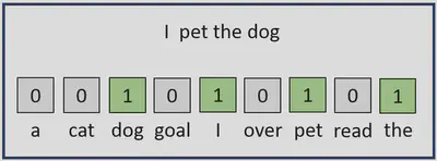
Let’s add another example to the one pictured above. Consider a corpus consisting of three documents:

1. Document1: “Karma is my boyfriend.”
2. Document2: “Karma is a god.”
3. Document3: “Karma is the breeze in my hair on the weekend.”

Then, the vocablary ($V$) is defined as: $$V = \begin{align}[ &\text{‘a’}, \text{‘boyfriend’}, \text{‘breeze’}, \text{‘god’}, \text{‘hair’}, \text{‘in’}, \\ &\text{‘is’}, \text{‘karma’}, \text{‘my’}, \text{‘on’}, \text{‘the’}, \text{‘weekend’} ]\end{align}$$

Our vocabulary is of length $12$, meaning that each vector resulting from our conversion will be of dimension $12$. To construct $v_1$, for example, we start by finding the position of the first word: ‘Karma’. The position is $8$, so $v_1[8] = 1$. Continuing this way, we end up with the following vectors:

$$ \begin{align} v_1 &= [0,1,0,0,0,0,1,1,1,0,0,0] \\ v_2 &= [1,0,0,1,0,0,1,1,0,0,0,0] \\ v_3 &= [0,0,1,0,1,1,1,1,1,1,1,1]. \end{align} $$

So, at this point, we’ve achieved the goal we set for ourselves. We took text and converted it into machine learning digestible form. Mission accomplished. Why not call it a day? While simple and easy to implement, there are some clear drawbacks to what we did:

1. Frequency of words is not captured.
2. Not all words are created equal. We’ve lost any measure of the relative importance of words.
3. Some degree of semantics is lost.

Each of these observations will help motivate us through the two remaining methods: TF-IDF and word embeddings.

Term Frequency - Inverse Document Frequency

An easy way to address the first identified drawback involves only a simple tweak to the process. Instead of creating each vector by marking ones and zeros, simply mark position $j$ with the number of times word $j$ appears in the document. For example, Document 3 from our ‘Swifty’ example would now map to the following vector:

$$ v_3 = [0,0,1,0,1,1,1,1,1,1,2,1] $$

Notice, we’ve adjusted the entry corresponding to ‘the’ to reflect it’s frequency within the document. It’s an improvement, but still lacking something important. Namely, we haven’t addressed the second identified drawback; not all words are created equal! The word ‘is’ appears in each of the three documents and so, in some sense, carries with it less information than the word, ‘breeze’, only appearing in Document 3. That’s the key insight that motivates the approach aptly named ‘term frequency - inverse document frequency’ or ‘tf-idf’.

One way to formalize this is as follows:

$$ \text{tfidf}(t,D,C) = \frac{\frac{f_{t,D}}{\sum_{t^\prime \in D}f_{t^\prime,D}}}{\log\left(\frac{|C|}{|\{D \in C: t \in D\}|}\right)} $$

where $t$, $D$ and $C$ symbolize terms, documents and a corpus, respectively. If that looks wonky, notice that the numerator is simply the relative within-document frequency of a term, while the denominator is a measure of the relative across-documents frequency. This gives us a leg up on simple, binary BoW vectors, but it still doesn’t do anything to address any lost semantics.

Word Embeddings

Synonyms exist; duh! Obvious, but, as of yet, missing from our formulations of $v_i$. More than that, words don’t have to be synonyms to be related. ‘King’ and ‘Queen’ definitely represent related concepts, but they aren’t synonymous, let alone the same word. Even using tf-idf, there’s no avenue for that information to travel down. What to do?

Well, certainly if words are synonymous, they’ll likely be used in similar ways. Namely, the words surrounding them will tend to also be related. Context is key! That’s an important insight that motivates embedding models like ‘Word2Vec’.

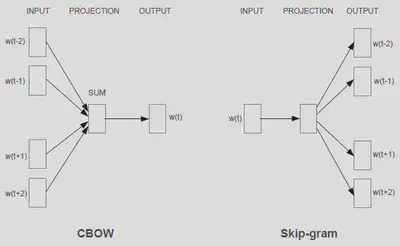
What does that mean in practice? Well, for Word2Vec, it could mean one of two things, each corresponding to a different model. In the first, given a document, we slide a context window of fixed length (say nine words) throughout. We then train the model to predict the middle (fifth) word, given the surrounding words (four previous and four subsequent). This describes the ‘Continuous Bag of Words’ (or CBOW) model.

Flipping the CBOW on it’s head gives us the second model, known as the ‘Skipgram’. Instead of predicting the word, given the context, we train a model to predict the context given the word. If that sounds strange, I’d recommend referencing the image below from Mikolov et al. 2013 and checking out Jay Alammar’s blog post: The Illustrated Word2Vec.

This works; i.e. it captures various different degrees of similarity and hence some level of semantics. Famously, we can take the embedding for the word ‘King’, subtract the embedding for the word ‘man’, add the embedding for the word ‘woman’ and the resulting vector will be very close to the embedding for the word ‘Queen’. Two distinct words and their relationship captured.

We can improve, still, upon Word2Vec. You’ll notice that while context is considered during training, it’s absent during scoring. In other words, if I score the same word three times, from three different sentences, Word2Vec will yield the same embedding. We call this being context independent. Since Word2Vec was published in 2013, further advancements have paved the way for context-dependent models like the RNN ELMo, and transformer based methods like BERT.

Similar to words, entire documents can be embedded into dense vectors and those are going to be crucial for the rest of the pipeline. Because of that, we need some kind of storage vehicle for these vectors. That’s exactly what vector stores are. In the next section, we’ll look at an example and how it can be utilized for efficient document retrieval.

Retrievers

Having done our preprocessing, we can now start to introduce the rest of the components within Docs2Chat’s various QA pipelines.

graph LR;
    A[(Vectorstore: Embeddings)]
    B[Retriever]
    C[Ranker]
    D[Reader]
    E[Generative Pipeline]
    F[Post-Processing]
    G[Response]

    A --> B

    B -->|if chain_type=search| C
    B -->|if chain_type=snip| D
    B -->|if chain_type=generative| E

    C & D & E --> F --> G

The third layer from the left (Reader, Ranker, Generative Pipeline) is where you might say “the magic happens”. That’s where, given a user query, we generate or extract (depending on the user’s chain_type specification) a response. But before we get to that, we have to go through the preceding layer. So what and why is a Retriever?

Similarity Search

Like the name suggests, a Retriever object retrieves documents thought to be relevant to a user query. We can think of it as a “short list” generator for our Reader/Ranker/Generative Pipeline. This is a common approach to designing what could potentially be very computationally intensive applications. Instead of running the complex algorithm on everything, we run a simpler one, first. The purpose of that being to generate a short list which we then run the more complicated algorithm on.

To be a little more concrete, the Reader/Ranker/Generative Pipeline is the “complicated algorithm” in our case. The “simple algorithm” can be implemented in a number of ways. As an example, we could measure the cosine similarity between vectors. Other common similarity measures include the euclidean inner product and $l^2$ norm.

$$ \begin{align} &\text{Euclidean Inner Product: }<\vec{x}, \vec{y}> &&= \sum x_i \cdot y_i \\ &\text{Cosine Similarity: }cos(\vec{x}, \vec{y}) &&= \frac{\vec{x} \cdot \vec{y}}{\lVert\vec{x}\rVert\lVert\vec{y}\rVert} \\ &l^2\text{ Norm: }d_{l^2}(\vec{x}, \vec{y}) &&= \sqrt{<(\vec{x} - \vec{y}), (\vec{x} - \vec{y})>} \end{align} $$

So given a user query, a retriever might follow a procedure like the following:

1. Generate a text embedding, $e$, for the query.
2. Calculate the similarity between $e$ and every vector in our vectorstore.
3. Return the vectors with the highest similarity scores.

That’s certainly an improvement over blindly applying the third layer of our diagram to every document, but it still doesn’t scale well. Dealing with an exhaustive set of comparisons for every query still gets us linear complexity with respect to the number of document chunks. In the next section, we’ll briefly discuss a family of techniques that can help us do even better, making our vector retrieval still more efficient and reducing the complexity from: $\text{O}(n)$ to $\text{O}(1)$.

Locality Sensitive Hashing

I said it’s common, right? Case in point, we’re going to rely on another “short list” generator to help us side-step an exhaustive search altogether. Namely, let’s discuss “locality sensitive hashing”.

Locality sensitive hashing (LSH) is a technique in which a hash function is developed that intentionally collides “similar” items with “high” probability. To be formal, consider the following:

• A collection of buckets, $S$.
• A metric space $\mathcal{M} = (M,d)$.
• A family of functions, $\mathcal{F}$ mapping $M \mapsto S$.
• Two real numbers $d_1 < d_2 \in \mathbb{R}$.
• Two probabilities $p_1, p_2 \in [0,1]$.

Then, we say $\mathcal{F}$ is $(d_1,d_2,p_1,p_2) - sensitive$ if for every $f \in \mathcal{F}$ and for all $x,y \in M$:

1. If $d(x,y) \leq d_1$, then $\mathbb{P}(f(x) = f(y)) \geq p_1$.
2. If $d(x,y) \geq d_2$, then $\mathbb{P}(f(x) = f(y)) \leq p_2$.

To be less formal, the idea is that more similar items should collide more often and less similar items shoud collide less often. A common example is implemented via a technique known as “MinHashing”. To not widen our scope too far, we’ll omit the technical details.

Both LangChain and Haystack implement vector stores and retriever objects of various kinds like “Elasticsearch” and FAISS (Facebook AI Similarity Search). In the case of Docs2Chat, we utilized the latter. Here are some resources, if you’re interested in diving deeper into the methodology and implementation:

• Paper: “Billion-scale similarity search with GPUs”
• Python Implementation: faiss-cpu
• Documentation: faiss.ai

Rankers: Bi-Encoders vs Cross-Encoders

What happens after retrieval depends on the ‘mode’ selected: namely, one of ‘search’, ‘snip’, or ‘generative’. In the case that the selected mode is ‘search’, we feed the retrieved documents to a ‘ranker’ or ’re-ranker' model. The point of a ranker model is likely exactly what you would expect. Namely, given a set of retrieved documents, a ranker re-orders them according to an estimate of relevance to the given query.

Naturally, you might wonder if this is duplicative; the whole point of a retriever was to return relevant documents using vector embeddings and similarity searches. At a high level, it is duplicative. The rationale for including it is simply for better performance. Rankers estimate relevancy using a different methodology than simple vector similarity search; one that tends to be more accurate, but also more computationally intensive. Putting this in more technical terms, the retrieval process described above is an example of a ‘bi-encoder’, while the ranking process will implement a ‘cross-encoder’.

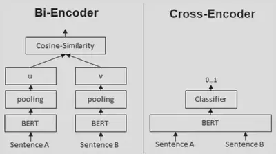
Take a look at the architectural differences between the two approaches, pictured above. Notice that with a cross-encoder, both documents must be passed into the model simultaneously, whereas, with bi-encoders, embeddings can be generated independently. That gives bi-encoders a huge computational advantage. Since we can generate embeddings for our repository of documents during preprocessing, that means at inference time, all that’s left to do is to generate the query embeddings and compute a similarity measure. I.e. our LLM only performs inference once, per query. A cross-encoder, by comparison would require our LLM to perform inference $n$ times (assuming our repository contains $n$ documents).

Just like before when we were discussing retrievers, we have a relatively accurate process that is computationally intensive and a relatively computationally cheap process that may be less accurate. Thus, also like before, we’ll utilize the computationally cheap option to generate a short list of answers and the accurate option to make a selection from said list. This is how and why we use both bi-encoders (retrievers) and cross-encoders (rankers).

Check below for an example of how to instantiate a ranker object and add it to a pipeline in Haystack.

from haystack.nodes import SentenceTransformersRanker
from haystack.pipelines import ExtractiveQAPipeline, Pipeline


# Instantiate the Ranker.
ranker = SentenceTransformersRanker(
    model_name_or_path="cross-encoder/ms-marco-MiniLM-L-12-v2",
)

# Create a pipeline consisting of a retriever and ranker.
hs_pipeline = Pipeline()
hs_pipeline.add_node(
    component=retriever, name="Retriever", inputs=["Query"]
)
hs_pipeline.add_node(
    component=ranker, name="Ranker", inputs=["Retriever"]
)

Once the retrieved documents are run through the ranker, we return the top scoring result as the ‘search’ result. That means,‘search’ mode in Docs2Chat simply returns the document chunk with the highest estimated query relevance. Since we’re returning an extracted portion of one of the source docuements, this is an example of an extractive pipeline (compared to generative). In the next section, we’ll see another example of an extractive pipeline, before, finally discussing ‘generative’ pipelines.

Readers

If we want to be more precise than simply returning a premade document chunk, we can set the chain_type to ‘snip’. Instead of returning an entire chunk, this selects and returns a text span. In other words, it tries to ‘snip’ out only the most relevant portion of a document chunk.

In Haystack, readers are objects that use LLMs to implement SQuAD and Google Natural Question style QA. In particular, they support using BERT-based models: BERT, RoBERTa, ALBERT, etc.. Of the three reader classes that Haystack offers (FARMREader, TransformersReader and TableReader), Docs2Chat uses the FARMReader and, in general, it seems like it is the easier of the two non-table readers to work with in Haystack. Fine-tuning, for example can be done relatively easily too, although, I admittedly haven’t played much with this yet. To create a QA pipeline using a reader, we can use the ExtractiveQAPipeline object.

from haystack.nodes import FARMReader
from haystack.pipelines import ExtractiveQAPipeline


reader = FARMReader("deepset/roberta-base-squad2")
hs_pipeline = ExtractiveQAPipeline(reader, retriever)

For more information, check the Haystack docs for Readers and ExtractiveQAPipeline.

Generative Pipelines

While powerful and the natural fit for plenty of use-cases, extractive pipelines generally aren’t the one’s making most of today’s headlines. Models like those that underpin ChatGPT and Bing Chat don’t just rank or snip documents, they generate new content. This enables exchanges that feel conversational. When it’s working well, it can seem like magic, but at it’s core, all these models are doing is next-word (or, more accurately, next-token) prediction. In other words, consider the following text:

“Even though he wanted to be early, Kevin got a flat tire and wound up arriving …”

We know the next word should probably be “late” and it’s precisely that type of knowledge that generates flashy feats like those generated by the aforementioned chat apps. The model guesses what the next word should be, uses that guess to then make a subsequent guess, uses that guess to make another subsequent guess and before you know it, you’ve got a full response.

In LangChain, we can utilize LLMs for generative pipelines by taking advantage of the ConversationalRetrievalChain object, for example.

from langchain.memory import ConversationBufferMemory
from langchain.chains import ConversationalRetrievalChain
from langchain.llms import LlamaCpp


# Load Llama2.
llm = LlamaCpp(
    model_path=config_obj.MODEL_PATH,
    n_ctx=2048,
    input={"temperature": 0.75, "max_length": 2000, "top_p": 1},
    verbose=False
)

# Instantiate memory object.
memory = ConversationBufferMemory(
    memory_key="chat_history",
    return_messages=True,
    output_key="answer"
)

# Define LLM pipeline.
ConversationalRetrievalChain.from_llm(
    llm=llm,
    retriever=vectorstore.as_retriever(),
    memory=memory, 
    return_source_documents=True
)

In the above code-snippet, we’re loading a Llama2 model as our llm, instantiating a memory object and creating a generative pipeline via the ConversationalRetrievalChain.from_llm method call. The memory object enables the model to reference previous exchanges when generating responses. Suppose I ask: “Who is the fastest human being alive?” and subsequent to the response, I ask “What country are they from?”. Adding memory gives the model the tools to figure out that when we use the pronoun “they”, we’re referring to “the fastest human being alive”.

And now, we have all of the pieces necessary to build some powerful LLM applications. We’ve covered LangChain & Haystack, document loading & splitting, converting text to vectors, vectorstores & retrievers and extractive and generative “retriever-augmented” pipelines. Docs2Chat combines all of this in the form of a CLI application and take a look at how to use it at the end of this post.

LLM Pipeline Use-Cases

Why is it useful? Hopefully, you already thought or I managed to convince you that the modern NLP landscape is exciting and engaging simply in and of itself, but what are the practical applications? Why would someone want to adopt Docs2Chat or a similar type of application in their personal life, or for their business?

Imagine boosting your and/or your organization’s efficiency by enabling quick, robust search? In the age of information, knowledge itself is rarely the bottleneck for productivity. Instead, the impediment to quick progress is often locating the right pieces of knowledge. One way in which large language model pipelines showcase their utility is by enabling such robust semantic searches. Searchability streamlines the onboarding process, helps developers find the right documentation and tools, empowers quick sifting through legal documents, etc.. Not having to spend more time finding the information you need than you do using that information frees time previously bogged down.

When we have information and know where it is, sometimes the bottleneck becomes time. Reading through all relevant documents isn’t always a feasible option. A RAG pipeline utilizing a model for summarization, for example, can help distill crucial pieces of information from long documents while giving you back the time you need to do the rest of your job, hobbie, etc..

In summary, retrieval augmented LLM pipelines can be great tools for helping people and organizations navigate the flood of information that comes with living in the age of information. In the next section, we’ll walk through the steps for installing and using Docs2Chat.

CLI Application

Combining the components we’ve outlined in the previous sections and bundling them in the form of a CLI app gives us Docs2Chat. The application is designed to allow users to query documents of their choosing without having to make any API calls to third parties. Here’s a quick overview of how to set it up and run.

1. Clone the repository: git clone https://github.com/BobbyLumpkin/docs2chat.git.

2. Create a documents directory at the main project level and add any and all documents you want the model to be able to access for it’s responses.

3. Create a models directory and download the appropriate models there. Example models:

   • Embedding Model: sentence-transformers/all-MiniLM-L6-v2
   • Ranking Model: cross-encoder/ms-marco-MiniLM-L-12-v2
   • Reader Model: deepset/roberta-base-squad2
   • Generative Model: TheBloke/Llama-2-7B-Chat-GGML

4. Install the Docs2Chat Python package: python -m pip install .

5. Run the application using the docs2chat entrypoint and specifying chain_type.

   • The chain_type can be one of search, snip or generative and corresponds to the paradigms we’ve discussed by the same name, in previous sections.

Search (docs2chat --chain_type="search")

This implements the retriever-ranker design, returning the entire document chunks thought to be most relevant to the query.

Snip (docs2chat --chain_type="snip")

This implements the retriever-reader design, returning a snipped out portion of a document chunk thought to contain the most query relevant content.

Generative (docs2chat --chain_type="generative")

This implements retriever-augmented generation (or RAG), producing query responses in a conversational form.

And if you’ve made it this far, I hope you got something out of it and thanks for reading!

References

[1] Alammar, J. (n.d.). The Illustrated Word2vec. Jalammar.github.io. http://jalammar.github.io/illustrated-word2vec/

[2] Devlin, J., Chang, M.-W., Lee, K., & Toutanova, K. (2018, October 11). BERT: Pre-training of Deep Bidirectional Transformers for Language Understanding. ArXiv.org. https://arxiv.org/abs/1810.04805

[3] Hu, Z. (n.d.). Question Answering on SQuAD with BERT. https://web.stanford.edu/class/archive/cs/cs224n/cs224n.1194/reports/default/15792151.pdf

[4] Johnson, J., Douze, M., & Jégou, H. (2017). Billion-scale similarity search with GPUs. ArXiv:1702.08734 [Cs]. https://arxiv.org/abs/1702.08734

[5] Kwiatkowski, T., Palomaki, J., Redfield, O., Collins, M., Parikh, A., Alberti, C., Epstein, D., Polosukhin, I., Devlin, J., Lee, K., Toutanova, K., Jones, L., Kelcey, M., Chang, M.-W., Dai, A. M., Uszkoreit, J., Le, Q., & Petrov, S. (2019). Natural Questions: A Benchmark for Question Answering Research. Transactions of the Association for Computational Linguistics, 7, 453–466. https://doi.org/10.1162/tacl_a_00276

[6] Mikolov, T., Chen, K., Corrado, G., & Dean, J. (2013, September 7). Efficient Estimation of Word Representations in Vector Space. ArXiv.org. https://arxiv.org/abs/1301.3781

[7] Rajpurkar, P., Jia, R., & Liang, P. (2018). Know What You Don’t Know: Unanswerable Questions for SQuAD. ArXiv:1806.03822 [Cs]. https://arxiv.org/abs/1806.03822

‌[8] Rajpurkar, P., Zhang, J., Lopyrev, K., & Liang, P. (n.d.). SQuAD: 100,000+ Questions for Machine Comprehension of Text. https://arxiv.org/pdf/1606.05250.pdf

[9] Haystack. (n.d.). Haystack. https://haystack.deepset.ai/

‌[10] LangChain. (n.d.). Www.langchain.com. https://www.langchain.com/

‌[11] SentenceTransformers Documentation — Sentence-Transformers documentation. (n.d.). Www.sbert.net. https://www.sbert.net/index.html